Uraz's R Blog: Monitor Central Banks Interest Rates

In the previous post, I shared a chart of central bank interest rates. We’ll see how we can customize the table on the site, which I’ve included below.

When we right-click on the page and select inspect, we can see that the data is in the table element below.

Using the table element makes scraping much simpler.

library(rvest)
library(dplyr)
library(stringr)
library(lubridate)
library(ggplot2)

url <- "https://www.cbrates.com/"

irs <- read_html(url) %>% 
  html_table()

The code above will generate a list in the environment when it is executed. The table we want to get to is the fourth item on the list.

master <- irs %>% 
  .[[4]]

The table is somewhat disorganized. The first 10 lines are provided below.

X1	X2	X3	X4
Worldwide Central Bank Rates	Worldwide Central Bank Rates	Worldwide Central Bank Rates	Worldwide Central Bank Rates
Subscribe to our Newsletter `/ Rate Alerts via Twitter / Donation to cbrates: paypal.com OECD & G20 Countries: </td>`	Subscribe to our Newsletter `/ Rate Alerts via Twitter / Donation to cbrates: paypal.com OECD & G20 Countries: </td>`	Subscribe to our Newsletter `/ Rate Alerts via Twitter / Donation to cbrates: paypal.com OECD & G20 Countries: </td>`	Subscribe to our Newsletter `/ Rate Alerts via Twitter / Donation to cbrates: paypal.com OECD & G20 Countries: </td>`
	75.00 % (+ 5.50)	Argentina \| Benchmark Rate (Sep 22, 2022)	Central Bank
	2.60 % (+ 0.25)	Australia \| Cash Rate (oct 04, 2022) - `CHART </td>`	Historical Rates
	13.75 % (+ 0.50)	Brazil \| Selic Rate (Aug 03, 2022)	Central Bank
	3.25 % (+ 0.75)	Canada \| Target ON Rate (Sep 07, 2022) - `CHART </td>`	Historical Rates
	10.75 % (+ 1.00)	Chile \| Monetary Policy Rate (Sep 06, 2022)	Central Bank
	3.65 % (- 0.05)	China \| Loan Prime Rate, LPR (Aug 22, 2022)	Central Bank
	10.00 % (+ 1.00)	Colombia \| Key Policy Rate (Sep 29, 2022)	Central Bank
	8.50 % (+ 1.00)	Costa Rica \| Policy Rate (Sep 14, 2022)	Central Bank

It’s time to put our hand on the table.

The first two lines can be removed as they won’t work for us.

master <- master %>% 
  slice(-c(1,2))

X2	X3	X4
75.00 % (+ 5.50)	Argentina \| Benchmark Rate (Sep 22, 2022)	Central Bank
2.60 % (+ 0.25)	Australia \| Cash Rate (oct 04, 2022) - `CHART </td>`	Historical Rates
13.75 % (+ 0.50)	Brazil \| Selic Rate (Aug 03, 2022)	Central Bank
3.25 % (+ 0.75)	Canada \| Target ON Rate (Sep 07, 2022) - `CHART </td>`	Historical Rates
10.75 % (+ 1.00)	Chile \| Monetary Policy Rate (Sep 06, 2022)	Central Bank

The first and fourth column can be removed.

master <- master %>% 
  select(-c(1,4))

X2	X3
75.00 % (+ 5.50)	Argentina \| Benchmark Rate (Sep 22, 2022)
2.60 % (+ 0.25)	Australia \| Cash Rate (oct 04, 2022) - `CHART </td>`
13.75 % (+ 0.50)	Brazil \| Selic Rate (Aug 03, 2022)
3.25 % (+ 0.75)	Canada \| Target ON Rate (Sep 07, 2022) - `CHART </td>`
10.75 % (+ 1.00)	Chile \| Monetary Policy Rate (Sep 06, 2022)

We’ll extract five pieces of information from the final version of the above table: Country, date of interest rate decision, interest rate, basis point, and sign.

The countries in the second column appear before the “|” symbol, and we can easily extract them using the stringr package’s word() function.

master <- master %>% 
  mutate(
    "Country" = word(X3,1,sep = "\\|")
  )

X2	X3	Country
75.00 % (+ 5.50)	Argentina \| Benchmark Rate (Sep 22, 2022)	Argentina
2.60 % (+ 0.25)	Australia \| Cash Rate (oct 04, 2022) - `CHART </td>`	Australia
13.75 % (+ 0.50)	Brazil \| Selic Rate (Aug 03, 2022)	Brazil
3.25 % (+ 0.75)	Canada \| Target ON Rate (Sep 07, 2022) - `CHART </td>`	Canada
10.75 % (+ 1.00)	Chile \| Monetary Policy Rate (Sep 06, 2022)	Chile

The dates of interest decisions can be extracted from the same column. The important thing to understand is how to get a string inside parentheses. After obtaining the strings in parentheses, the values can be converted to date format using the lubridate package’s mdy() function.

# master <- master %>% 
#   mutate(
#     "DecisionDate" = gsub("[\\(\\)]", "", regmatches(X3, gregexpr("\\(.*?\\)", X3))),
#     "DecisionDate" = mdy(DecisionDate)
#   )

# OR

master <- master %>% 
  mutate(
    "DecisionDate" = mdy(gsub("[\\(\\)]", "", regmatches(X3, gregexpr("\\(.*?\\)", X3))))
  )

X2	X3	Country	DecisionDate
75.00 % (+ 5.50)	Argentina \| Benchmark Rate (Sep 22, 2022)	Argentina	2022-09-22
2.60 % (+ 0.25)	Australia \| Cash Rate (oct 04, 2022) - `CHART </td>`	Australia	2022-10-04
13.75 % (+ 0.50)	Brazil \| Selic Rate (Aug 03, 2022)	Brazil	2022-08-03
3.25 % (+ 0.75)	Canada \| Target ON Rate (Sep 07, 2022) - `CHART </td>`	Canada	2022-09-07
10.75 % (+ 1.00)	Chile \| Monetary Policy Rate (Sep 06, 2022)	Chile	2022-09-06

The word() function can still be used to obtain interest rates from the first column.

master <- master %>% 
  mutate(
    "InterestRate" = word(X2,1,1)
  )

X2	X3	Country	DecisionDate	InterestRate
75.00 % (+ 5.50)	Argentina \| Benchmark Rate (Sep 22, 2022)	Argentina	2022-09-22	75.00
2.60 % (+ 0.25)	Australia \| Cash Rate (oct 04, 2022) - `CHART </td>`	Australia	2022-10-04	2.60
13.75 % (+ 0.50)	Brazil \| Selic Rate (Aug 03, 2022)	Brazil	2022-08-03	13.75
3.25 % (+ 0.75)	Canada \| Target ON Rate (Sep 07, 2022) - `CHART </td>`	Canada	2022-09-07	3.25
10.75 % (+ 1.00)	Chile \| Monetary Policy Rate (Sep 06, 2022)	Chile	2022-09-06	10.75

Finally, as in the second column, the strings in parentheses, i.e. basis points, can be obtained from the first column. We can find the base points by converting these values to numbers and multiplying them by 100. According to the standard basis point conversion, one percent of a percentage change equals one hundred basis points. As a result, the standard conversion will be, 100 basis points = 1% percentage change or 0.01% percentage change = 1 basis point.

master <- master %>% 
  mutate(
    "BasisPoint" = gsub("[\\(\\)]", "", regmatches(X2, gregexpr("\\(.*?\\)", X2)))
  )

X2	X3	Country	DecisionDate	InterestRate	BasisPoint
75.00 % (+ 5.50)	Argentina \| Benchmark Rate (Sep 22, 2022)	Argentina	2022-09-22	75.00	5.50
2.60 % (+ 0.25)	Australia \| Cash Rate (oct 04, 2022) - `CHART </td>`	Australia	2022-10-04	2.60	0.25
13.75 % (+ 0.50)	Brazil \| Selic Rate (Aug 03, 2022)	Brazil	2022-08-03	13.75	0.50
3.25 % (+ 0.75)	Canada \| Target ON Rate (Sep 07, 2022) - CHART	Canada	2022-09-07	3.25	0.75
10.75 % (+ 1.00)	Chile \| Monetary Policy Rate (Sep 06, 2022)	Chile	2022-09-06	10.75	1.00

Let’s get the “+” and “-” signs at the beginning of the points in the last column and remove them from the column. These signs will be used later. The stringr’s word() function will also come in handy here.

master <- master %>% 
  mutate(
    "Sign" = word(BasisPoint,1,1)
  )

X2	X3	Country	DecisionDate	InterestRate	BasisPoint
75.00 % (+ 5.50)	Argentina \| Benchmark Rate (Sep 22, 2022)	Argentina	2022-09-22	75.00	5.50
2.60 % (+ 0.25)	Australia \| Cash Rate (oct 04, 2022) - CHART	Australia	2022-10-04	2.60	0.25
13.75 % (+ 0.50)	Brazil \| Selic Rate (Aug 03, 2022)	Brazil	2022-08-03	13.75	0.50
3.25 % (+ 0.75)	Canada \| Target ON Rate (Sep 07, 2022) - CHART	Canada	2022-09-07	3.25	0.75
10.75 % (+ 1.00)	Chile \| Monetary Policy Rate (Sep 06, 2022)	Chile	2022-09-06	10.75	1.00

We can leave the columns in the table that will be useful to us.

master <- master %>% 
  select(3:7)

Country	DecisionDate	InterestRate	BasisPoint
Argentina	2022-09-22	75.00	5.50
Australia	2022-10-04	2.60	0.25
Brazil	2022-08-03	13.75	0.50
Canada	2022-09-07	3.25	0.75
Chile	2022-09-06	10.75	1.00

There are extra spaces in the Country and BasisPoint columns, as can be seen. We can get rid of them by using the str_squish() function from the stringr package.

master <- master %>% 
  mutate(
    Country = str_squish(Country),
    BasisPoint = str_squish(BasisPoint)
  )

Country	DecisionDate	InterestRate	BasisPoint
Argentina	2022-09-22	75.00	5.50
Australia	2022-10-04	2.60	0.25
Brazil	2022-08-03	13.75	0.50
Canada	2022-09-07	3.25	0.75
Chile	2022-09-06	10.75	1.00

Let’s just leave the points in the BasisPoint column.

# master <- master %>% 
#   mutate(
#     BasisPoint = word(BasisPoint,2,2),
#     BasisPoint = as.numeric(BasisPoint)
#   )

# OR

master <- master %>% 
  mutate(
    BasisPoint = as.numeric(word(BasisPoint,2,2))
  )

Country	DecisionDate	InterestRate	BasisPoint
Argentina	2022-09-22	75.00	5.50
Australia	2022-10-04	2.60	0.25
Brazil	2022-08-03	13.75	0.50
Canada	2022-09-07	3.25	0.75
Chile	2022-09-06	10.75	1.00

If the Sign column is positive, we can multiply the values in the BasisPoint column by 100, and if negative, we can multiply by -100 to find the basis points.

master <- master %>% 
  mutate(
    BasisPoint = case_when(
      Sign == "+" ~ BasisPoint * 100,
      Sign == "-" ~ BasisPoint * (-100)
    )
  )

Country	DecisionDate	InterestRate	BasisPoint
Argentina	2022-09-22	75.00	550
Australia	2022-10-04	2.60	25
Brazil	2022-08-03	13.75	50
Canada	2022-09-07	3.25	75
Chile	2022-09-06	10.75	100

The line in the Country column that says Other Countries: can be removed because it is meaningless.

master <- master %>% 
  filter(Country != "Other Countries:")

Country	DecisionDate	InterestRate	BasisPoint
Argentina	2022-09-22	75.00	550
Australia	2022-10-04	2.60	25
Brazil	2022-08-03	13.75	50
Canada	2022-09-07	3.25	75
Chile	2022-09-06	10.75	100

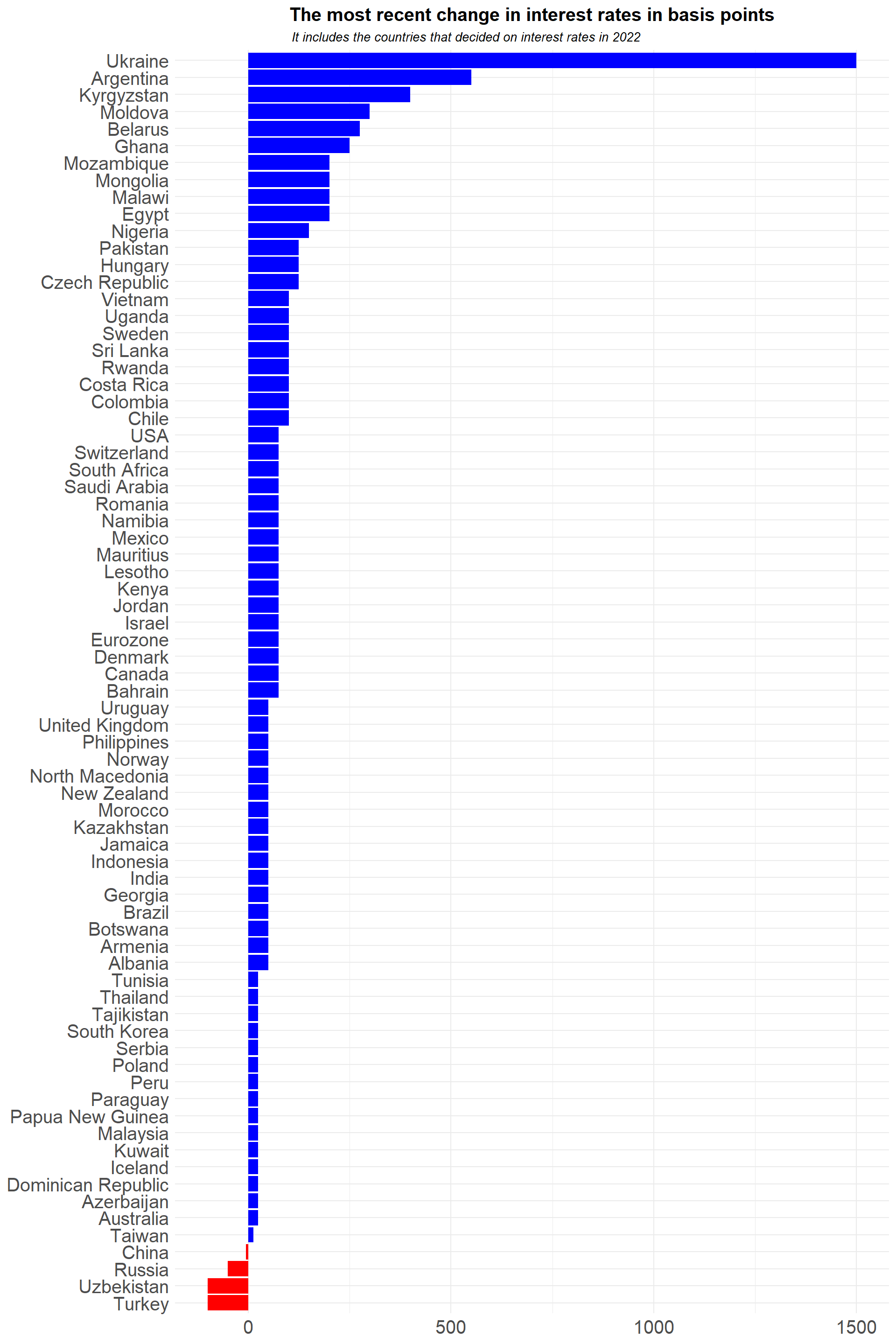
Finally, it’s time to visualize the data.

master %>% 
  filter(DecisionDate >= as.Date("2022-01-01")) %>% 
  ggplot(aes(x = reorder(Country, BasisPoint), y = BasisPoint, fill = Sign)) +
  geom_col(show.legend = FALSE) +
  coord_flip() +
  theme_minimal() +
  theme(axis.title = element_blank(),
        plot.title = element_text(face = "bold", size = 15, hjust = 0.5),
        plot.subtitle = element_text(face = "italic", size = 10, hjust = 0.32),
        axis.text = element_text(size = 15)) +
  scale_fill_manual(values = c("red","blue")) +
  labs(
    title = "The most recent change in interest rates in basis points",
    subtitle = "It includes the countries that decided on interest rates in 2022"
  )