According to the information I obtained from this website, the central banks of the countries that raised and cut interest rates in 2022 are shown below.
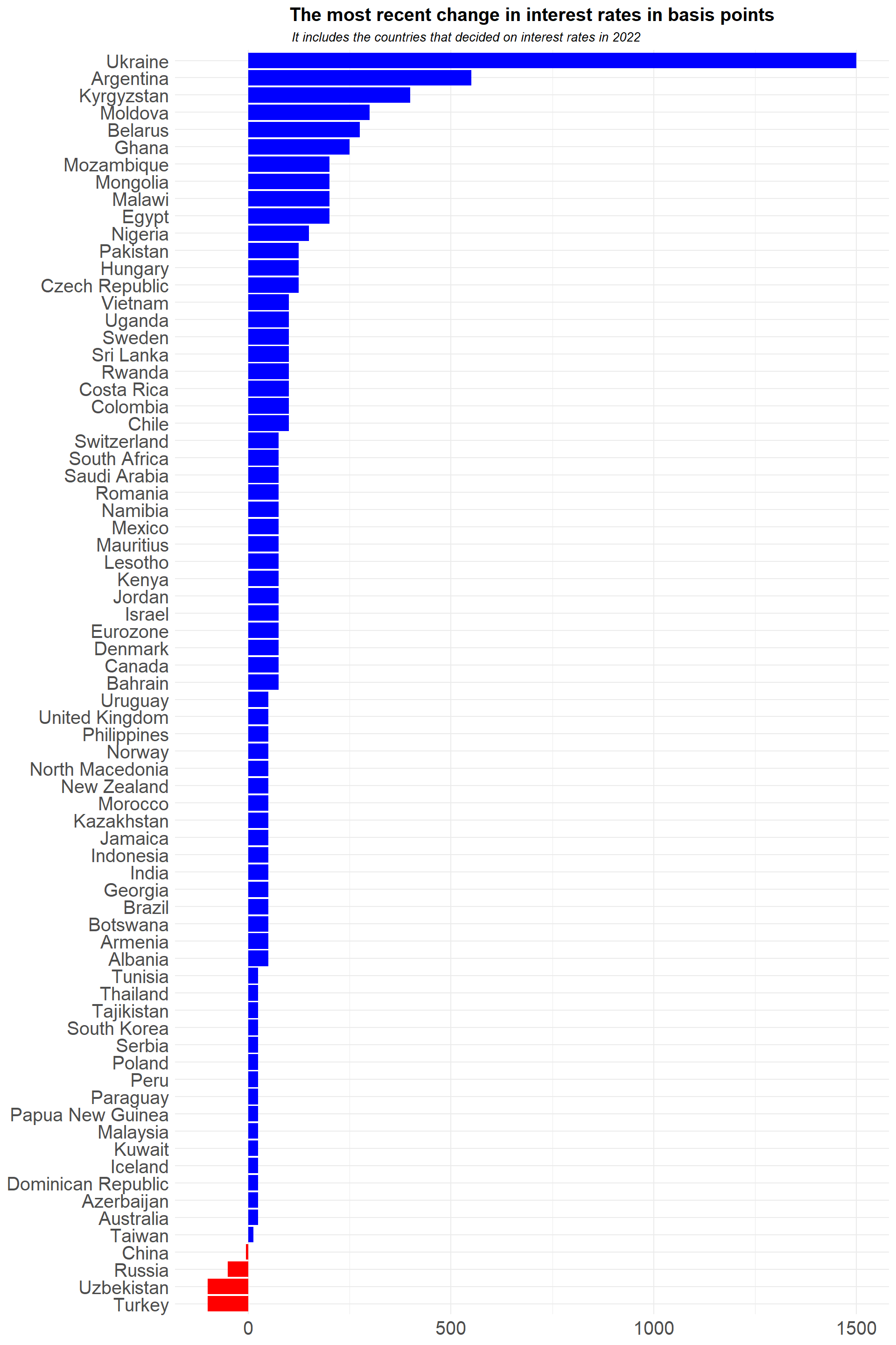
Only 4 of the 73 central banks that made interest rate decisions in 2022 decided to cut rates, according to the list. China, Russia, Uzbekistan, and Turkey are among them.
Interest rates play an important role in determining the value of a currency. As a result, I’d like to demonstrate how the USDTRY reacts to interest rate decisions made by the CBRT. The data you can access by downloading the post37.xlsx file from here is from Reuters.
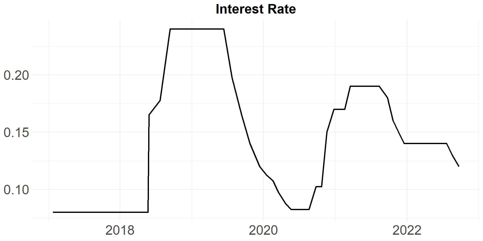
The rates for the USDTRY and historical interest rates are shown separately below.

If we normalize the data in the 0-1 range and combine the two variables, we get the following.

We can now look at how the CBRT’s interest rate decisions affect the USDTRY.
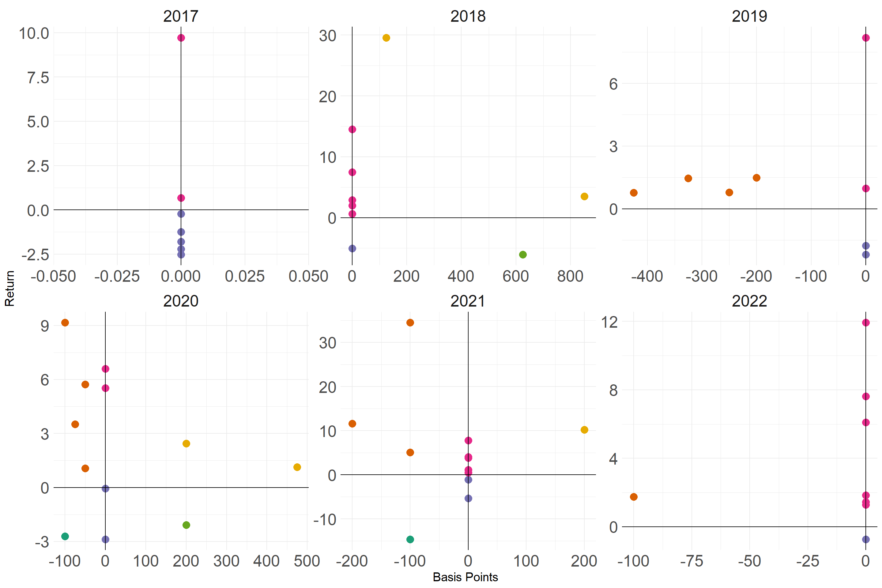
If we summarize the above graph;

| Status | N |
|---|---|
| IR Keeps Constant; ER Up | 22 |
| IR Keeps Constant; ER Down | 13 |
| IR Cuts; ER Up | 12 |
| IR Raises; ER Up | 5 |
| IR Cuts; ER Down | 2 |
| IR Raises; ER Down | 2 |
It seems that the CBRT will continue to cut interest rates in the coming months. As of 2017, the Turkish Lira depreciated until the next interest rate cut decision by the CBRT in 12 of the 14 cases.
If we visualize the movements of USDTRY with an initial value of 100 until the next CBRT interest rate decision, we get the following result.
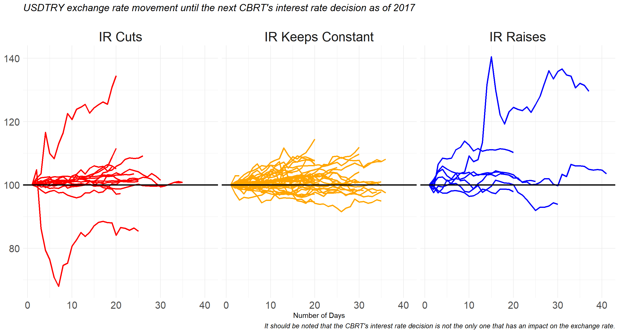
I’d like to remind you that, while variable interest rates can have an impact on exchange rates, domestic risks can also have an impact. Furthermore, the government is spending billions of dollars to suppress the USDTRY.
The codes that were used in the post are given below.
library(rvest)
library(tidyverse)

url <- "https://www.cbrates.com/"

df <- read_html(url) %>%
  html_table() %>%
  .[[4]] %>%
  slice(-c(1:2)) %>%
  select(-c(1,4)) %>%
  mutate(
    "Date" = lubridate::mdy(gsub("[\\(\\)]", "", regmatches(X3, gregexpr("\\(.*?\\)", X3)))),
    "Country" = str_squish(word(X3,1,sep = "\\|")),
    "Interest Rate" = as.numeric(word(X2,1,1)),
    "Bps" = str_squish(gsub("[\\(\\)]", "", regmatches(X2, gregexpr("\\(.*?\\)", X2)))),
    "Direction" = word(Bps,1,1),
    "Bps" = as.numeric(word(str_squish(gsub("[\\(\\)]", "", regmatches(X2, gregexpr("\\(.*?\\)", X2)))),2,2)),
    "Bps" = case_when(
      Direction == "+" ~ Bps*100,
      Direction == "-" ~ Bps*(-100)
    )
  ) %>%
  select(3:7) %>%
  na.omit() %>%
  filter(Date >= as.Date("2022-01-01"))

ggplot(df, aes(x = reorder(Country,Bps), y = Bps, fill = Direction)) +
  geom_col(show.legend = FALSE) +
  coord_flip() +
  theme_minimal() +
  theme(axis.title = element_blank(),
        plot.title = element_text(face = "bold", size = 15, hjust = 0.5),
        plot.subtitle = element_text(face = "italic", size = 10, hjust = 0.32),
        axis.text = element_text(size = 15)) +
  scale_fill_manual(values = c("red","blue")) +
  labs(
    title = "The most recent change in interest rates in basis points",
    subtitle = "It includes the countries that decided on interest rates in 2022"
  )

interest_rates <- readxl::read_excel("data.xlsx", sheet = "Policy Interest Rates") %>%
  mutate(
    date = lubridate::ymd(paste0(word(date,3,3)," ",word(date,2,2)," ",word(date,1,1)))
  ) %>%
  arrange(date)

ggplot(interest_rates, aes(x = date, y = policy_interest_rate)) +
  geom_line(size = 1) +
  theme_minimal() +
  theme(axis.title = element_blank(),
        axis.text = element_text(size = 20),
        plot.title = element_text(size = 20, face = "bold", hjust = 0.5)) +
  labs(
    title = "Interest Rate"
  )

usdtry_rates <- readxl::read_excel("data.xlsx", sheet = "USDTRY") %>%
  mutate(date = as.Date(date)) %>%
  arrange(date)

ggplot(usdtry_rates, aes(x = date, y = usdtry)) +
  geom_line(size = 1) +
  theme_minimal() +
  theme(axis.title = element_blank(),
        axis.text = element_text(size = 20),
        plot.title = element_text(size = 20, face = "bold", hjust = 0.5)) +
  labs(
    title = "USDTRY"
  )

normalized <- function(x){

  (x - min(x)) / (max(x) - min(x))

}

df_join <- interest_rates %>%
  left_join(usdtry_rates, by = "date") %>%
  rename(
    "Interest Rate"=2,
    "USDTRY"=3
  ) %>%
  mutate_at(
    vars(-date), function(x) normalized(x)
  ) %>%
  pivot_longer(!date, names_to = "vars", values_to = "vals")

ggplot(df_join, aes(x = date, y = vals, group = vars, color = vars)) +
  geom_line(size = 1) +
  theme_minimal() +
  theme(legend.title = element_blank(),
        legend.position = "top",
        legend.text = element_text(size = 20),
        legend.key.width = unit(3,"cm"),
        axis.title = element_blank(),
        axis.text.y = element_blank(),
        axis.text.x = element_text(size = 20)) +
  scale_color_manual(values = c("red","blue"))

master <- usdtry_rates %>%
  left_join(interest_rates, by = "date")

changes <- data.frame(
  "DecisionDate" = interest_rates$date[-nrow(interest_rates)],
  "InterestRates" = interest_rates$policy_interest_rate[-nrow(interest_rates)],
  "FirstER" = NA,
  "SecondER" = NA
)

firstER <- NULL
secondER <- NULL

for(i in 1:nrow(master)){

  if(!(is.na(master$policy_interest_rate[i]))){

    firstER <- c(firstER,master$usdtry[i])
    secondER <- c(secondER,master$usdtry[(i-1)])

  }

  if(i == nrow(master)){
      firstER <- firstER[-length(firstER)]
      changes$FirstER <- firstER
      changes$SecondER <- secondER
      changes$Bps <- lag((lead(changes$InterestRates) - changes$InterestRates)*10000)
      changes$ER <- (changes$SecondER / changes$FirstER - 1) * 100

      changes <- changes %>%
        mutate(
          "Status" = case_when(
            Bps > 0 & ER > 0 ~ "IR Raises; ER Up",
            Bps > 0 & ER < 0 ~ "IR Raises; ER Down",
            Bps > 0 & ER == 0 ~ "IR Raises; ER Notr",
            Bps < 0 & ER < 0 ~ "IR Cuts; ER Down",
            Bps < 0 & ER > 0 ~ "IR Cuts; ER Up",
            Bps < 0 & ER == 0 ~ "IR Cuts; ER Notr",
            Bps == 0 & ER > 0 ~ "IR Keeps Constant; ER Up",
            Bps == 0 & ER < 0 ~ "IR Keeps Constant; ER Down",
            Bps == 0 & ER == 0 ~ "IR Keeps Constant; ER Notr"

          )
        ) %>%
        na.omit() %>%
        mutate(
          "Year" = format(DecisionDate,"%Y")
        )

    }

}

changes %>%
  ggplot(aes(x = Bps, y = ER, color = Status)) +
  geom_point(size = 4, show.legend = FALSE) +
  geom_vline(xintercept = 0) +
  geom_hline(yintercept = 0) +
  theme_minimal() +
  labs(
    x = "Basis Points",
    y = "Return"
  ) +
  theme(strip.text = element_text(size = 20),
        axis.text = element_text(size = 20),
        axis.title = element_text(size = 15)) +
  scale_color_brewer(palette = "Dark2") +
  facet_wrap(~Year, scales = "free")

changes %>%
  group_by(Status) %>%
  summarise(N = n()) %>%
  ggplot(aes(x = reorder(Status, N), y = N, fill = N)) +
  geom_col(show.legend = FALSE) +
  coord_flip() +
  scale_fill_gradient(low = "orange", high = "red") +
  theme_minimal() +
  theme(axis.title = element_blank(),
        axis.text = element_text(size = 15))

master <- usdtry_rates %>%
  left_join(interest_rates, by = "date") %>%
  mutate(date = as.Date(date))

master$group <- NA

k <- 0

for(j in 1:nrow(master)){

  date <- master$date[j]

  if(date %in% interest_rates$date){

    master$group[j] <- paste0("G",k)
    k = k + 1

  }

  if(j == nrow(master)){

    master <- master %>%
      mutate(group = zoo::na.locf(group)) %>%
      filter(date >= as.Date("2017-03-16")) %>%
      rename("DecisionDate"=1) %>%
      left_join(changes[,c(1,7,8)], by = "DecisionDate") %>%
      mutate(Status = word(Status,1,sep = "\\;"),
             Status = zoo::na.locf(Status),
             Year = zoo::na.locf(Year)) %>%
      group_by(group) %>%
      mutate(RN = row_number()) %>%
      filter(DecisionDate != interest_rates$date[nrow(interest_rates)]) %>%
      ungroup()

    master2 <- data.frame()

    for(m in 1:nrow(changes)){

      group_filtered <- master %>%
        filter(group == paste0("G",m))

      minDateER <- group_filtered %>%
        filter(DecisionDate == min(DecisionDate)) %>%
        pull(usdtry)

      group_filtered$initialValue <- minDateER
      group_filtered$index <- group_filtered$usdtry / group_filtered$initialValue * 100

      master2 <- master2 %>%
        bind_rows(group_filtered)

    }

  }

}

ggplot(master2, aes(x = RN, y = index, group = group, color = Status)) +
  geom_line(size = 1, show.legend = FALSE) +
  geom_hline(yintercept = 100, size = 1) +
  theme_minimal() +
  theme(axis.title.y = element_blank(),
        axis.text = element_text(size = 15),
        plot.title = element_text(size = 15, face = "italic"),
        plot.caption = element_text(size = 10, face = "italic"),
        strip.text = element_text(size = 20)) +
  scale_color_manual(values = c("red","orange","blue")) +
  facet_wrap(~Status) +
  labs(
    title = "USDTRY exchange rate movement until the next CBRT's interest rate decision as of 2017",
    subtitle = "",
    x = "Number of Days",
    caption = "It should be noted that the CBRT's interest rate decision is not the only one that has an impact on the exchange rate."
  )