The volatility of a stock in relation to the overall market is measured by beta (\(\beta\)). The market, such as the BIST100 Index, has a beta of 1.0 by definition, and individual stocks are ranked based on how much they deviate from the market.
\(\beta = \frac{cov(R_e,R_m)}{var(R_m)}\)
\(\beta:\) Beta coefficient
\(R_e:\) The return on an individual stock
\(R_m:\) The return on the overall market
\(cov(R_e,R_m):\) How changes in a stock’s returns are related to changes in the market’s returns.
\(var(R_m):\) How far the market’s data points spread out from their average value
Regression analysis is used to calculate beta. The beta coefficient can be interpreted as follows:
\(\beta > 1:\) High Correlation, Higher Volatility
\(\beta = 1:\) High Correlation, Same Volatility
\(\beta < 1 > 0\ or\ 0\ to\ 1:\) Slight Correlation, Lower Volatility
\(\beta = 0:\) No Correlation
\(\beta > -1 < 0\ or\ -1\ to\ 0:\) Slight Inverse Correlation, Lower Volatility
\(\beta = -1:\) High Inverse Correlation, Same Volatility
\(\beta < -1:\) High Inverse Correlation, Higher Volatility
The data you can access by downloading the post35.xlsx file from here is from Reuters.
bist30 <- readxl::read_excel("data.xlsx")
Consider a stock and a market index. To build a regression model, we’ll use stock returns as the dependent variable and market index returns as the independent variable.
Let’s start with the daily returns.
We can now build the regression models.
betas <- data.frame(
  ticker = rep(unique(master$TICKER), each = length(unique(master$YEAR))),
  year = rep(unique(master$YEAR), length(unique(master$TICKER))),
  beta = NA
)

for(i in 1:nrow(betas)) {

  ticker <- betas$ticker[i]
  year <- betas$year[i]

  df_model <- master %>%
    filter(TICKER == ticker & YEAR == year) %>%
    na.omit()

  model <- lm(df_model$Return ~ df_model$XU100)
  beta <- model$coefficients[2]

  betas$beta[i] <- beta

}
I’d like to show the year-based betas of the stocks we are studying on.
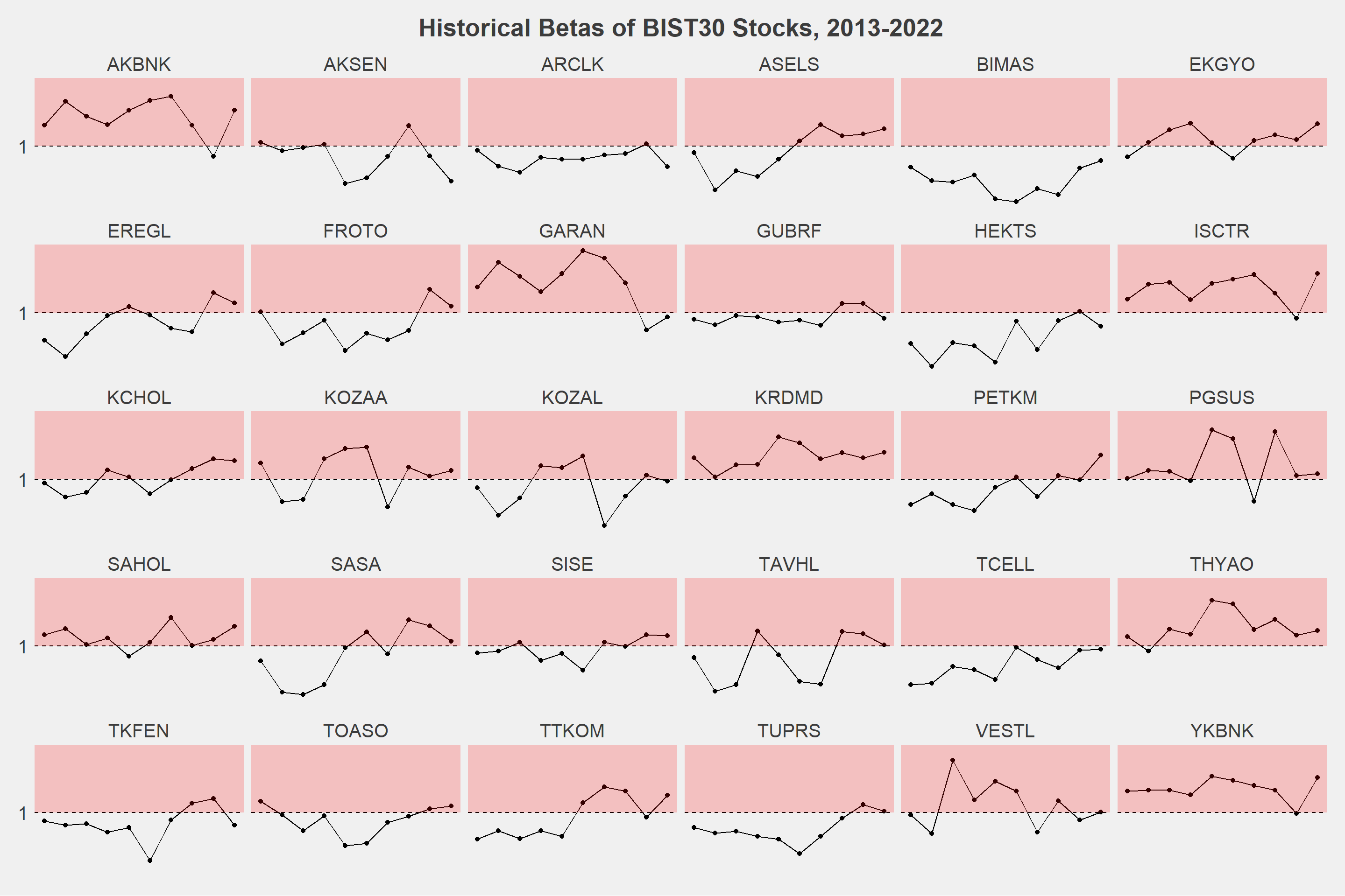
Let’s rank the stocks’ betas for 2022.

The codes for the last two data visualizations are provided below.
betas %>%
  ggplot(aes(x = year, y = beta)) +
  geom_line() +
  geom_point() +
  geom_hline(yintercept = 1, linetype = "dashed") +
  facet_wrap(~ticker) +
  ggthemes::theme_fivethirtyeight() +
  theme(strip.text = element_text(size = 15),
        plot.title = element_text(size = 20, hjust = 0.5),
        axis.text.y = element_text(size = 15),
        axis.text.x = element_blank(),
        panel.grid.major = element_blank()) +
  scale_y_continuous(breaks = c(0,1)) +
  labs(title = "Historical Betas of BIST30 Stocks, 2013-2022") +
  annotate(
    geom = "rect",
    xmin = -Inf,
    xmax = Inf,
    ymin = 1,
    ymax = Inf,
    fill = "red",
    alpha = .2
  )

betas %>%
  filter(year == 2022) %>%
  ggplot(aes(x = reorder(ticker, -beta), y = beta)) +
  geom_point(size = 5, alpha = .5) +
  ggrepel::geom_text_repel(aes(label = ticker), size = 7) +
  geom_hline(yintercept = 1, linetype = "dashed") +
  ggthemes::theme_fivethirtyeight() +
  theme(
    axis.text.x = element_blank(),
    panel.grid.major = element_blank(),
    axis.text.y = element_text(size = 15)
  ) +
  annotate(
    geom = "rect",
    xmin = -Inf,
    xmax = Inf,
    ymin = 1,
    ymax = Inf,
    fill = "red",
    alpha = .2
  )