Volatility can be measured in a variety of ways, and in this post I’d like to compare two of them.
The formulas for the two volatility methods mentioned in the title are shown below.
Close-to-Close Volatility:
Close-to-close historical volatility is calculated using only the closing prices of stocks.
\(\sigma_{cl} = \sqrt{\frac{1}{T-1}\sum_{t=1}^{T}(r_t-\bar{r})^2}\)
where:
\(T:\) Number of days in the sample period
\(r_t:\) Return on day t
\(\bar{r}:\) Mean return
High-Low or Parkinson Volatility:
Parkinson volatility is a measure of volatility that takes into account the stock’s high and low prices for the day.
\(\sigma_{hl} = \sqrt{\frac{1}{4Tln2}\sum_{t=1}^{T}ln(\frac{H_t}{L_t})^2}\)
where:
\(T:\) Number of days in the sample period
\(H_t:\) High price on day t
\(L_t:\) Low price on day t
We’ll use two methods to calculate the volatility of the stocks in the BIST30 index. The stock list is available on PDP, which stands for Public Disclosure Platform. The data were obtained from Reuters, which you can access by downloading the post34.xlsx file from here.
df <- readxl::read_excel("data.xlsx")

sampleSize <- nrow(df)
stockList <- unique(gsub("_Open|_High|_Low|_Close","",names(df)))[-1]
Close-to-Close Volatility:
close_to_close <- data.frame()

for(i in 1:31){

  cl <- df %>%
    select(contains(paste0(stockList[i],"_Close"))) %>%
    rename("Close"=1) %>%
    mutate(
      Return = lag(log(lead(Close) / Close)),
      Mean = mean(Return, na.rm = TRUE),
      ReturnMean2 = (Return - Mean)^2
    ) %>%
    pull(ReturnMean2) %>%
    sum(., na.rm = TRUE) / (sampleSize - 2) %>% # 31.12.2021 is not included & T - 1 = T - 2
    sqrt(.) * 100

  tbl_cl <- data.frame(
    "Ticker" = stockList[i],
    "ClosetoCloseVol" = cl
  )

  close_to_close <- close_to_close %>%
    bind_rows(tbl_cl)

}
High-Low or Parkinson Volatility:
high_low <- data.frame()

for(j in 1:31){

  hl <- df %>%
    select(contains(c(paste0(stockList[j],"_High"),paste0(stockList[j],"_Low")))) %>%
    rename("High"=1, "Low"=2) %>%
    mutate(HL = log(High/Low)^2) %>%
    pull(HL) %>%
    sum(.) / (4 * (sampleSize - 1) * log(2)) %>% # 31.12.2021 is not included = T - 1
    sqrt(.) * 100

  tbl <- data.frame(
    "Ticker"= stockList[j],
    "HighLowVol" = hl
  )

  high_low <- high_low %>%
    bind_rows(tbl)

}
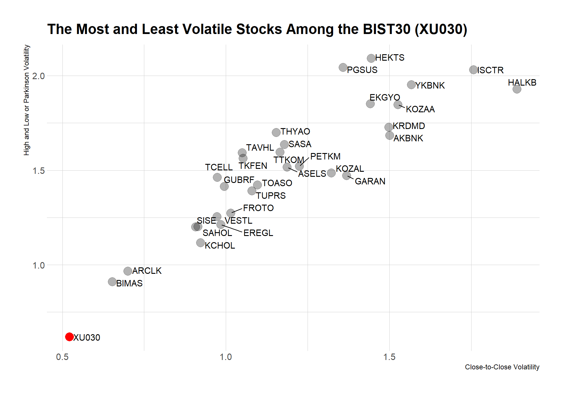
ggplot(master, aes(x = ClosetoCloseVol, y = HighLowVol)) +
  geom_point(size = 5, alpha = .3) +
  geom_point(data = master %>% filter(Ticker == "XU030"), color = "red", size = 5) +
  ggrepel::geom_text_repel(aes(label = Ticker), size = 4, nudge_x = 0.05) +
  hrbrthemes::theme_ipsum() +
  labs(
    title = "The Most and Least Volatile Stocks Among the BIST30 (XU030)",
    x = "Close-to-Close Volatility",
    y = "High and Low or Parkinson Volatility"
  )