A Look at Stock Market Performance After Elections: The Case of BIST100 Indices

Stock market performance by elections.

Turkey held general elections on the following dates (not included before 2002):

date	election
Nov 3, 2002	General
Jul 22, 2007	General
Jun 12, 2011	General
Jun 07, 2015	General
Nov 01, 2015	General
Jun 24, 2018	General

Since the AKP has been ruling Turkey since 2002, this work will actually be the government’s performance.

You can download the post32_1.xlsx and post32_2.xlsx files here or go to the CBRT’s website.

library(tidyverse)

bist100 <- readxl::read_excel("data1.xlsx") %>% 
  mutate(date = lubridate::dmy(date))

election_dates <- c("2002-11-03",
                    "2007-07-22",
                    "2011-06-12",
                    "2015-06-07",
                    "2015-11-01",
                    "2018-06-24")

ggplot(bist100, aes(x = date, y = close)) +
  geom_line() +
  geom_vline(xintercept = as.Date(election_dates), linetype = "dotdash", color = "red", size = 1) +
  ggthemes::theme_fivethirtyeight() +
  theme(axis.text = element_text(size = 20)) +
  scale_y_continuous(labels = scales::comma)

We’ll create indices starting with 100 using each election date as a start date.

# Groups

bist100 <- bist100 %>% 
  mutate(
    election = case_when(
      date >= as.Date("2002-11-03") & date < as.Date("2007-07-22") ~ "GE-1 (Nov 3, 2002)",
      date >= as.Date("2007-07-22") & date < as.Date("2011-06-12") ~ "GE-2 (Jul 22, 2007)",
      date >= as.Date("2011-06-12") & date < as.Date("2015-06-07") ~ "GE-3 (Jun 12, 2011)",
      date >= as.Date("2015-06-07") & date < as.Date("2015-11-01") ~ "GE-4 (Jun 07, 2015)",
      date >= as.Date("2015-11-01") & date < as.Date("2018-06-24") ~ "GE-5 (Nov 01, 2015)",
      date >= as.Date("2018-06-24") ~ "GE-6 (Jun 24, 2018)"
    )
  )

# Initial Values

initialValues <- bist100 %>% 
  group_by(election) %>% 
  slice_min(date) %>% 
  rename("initial"=2) %>% 
  ungroup()

# Indices

master <- bist100 %>% 
  left_join(initialValues, by = c("date","election")) %>% 
  mutate(initial = zoo::na.locf(initial), # Replace NAs with previous value
         "indices" = close / initial * 100) %>% 
  group_by(election) %>% 
  mutate(t = row_number()) %>% 
  ungroup()

Done!

ggplot(master, aes(x = t, y = indices)) +
  geom_line(data = master %>% rename(election2 = election),
            aes(group = election2), color = "gray", size = 1) +
  geom_line(color = "dark blue", size = 1.5) +
  ggthemes::theme_fivethirtyeight() +
  theme(strip.text = element_text(size = 20),
        axis.text = element_text(size = 20)) +
  facet_wrap(~election, ncol = 2)

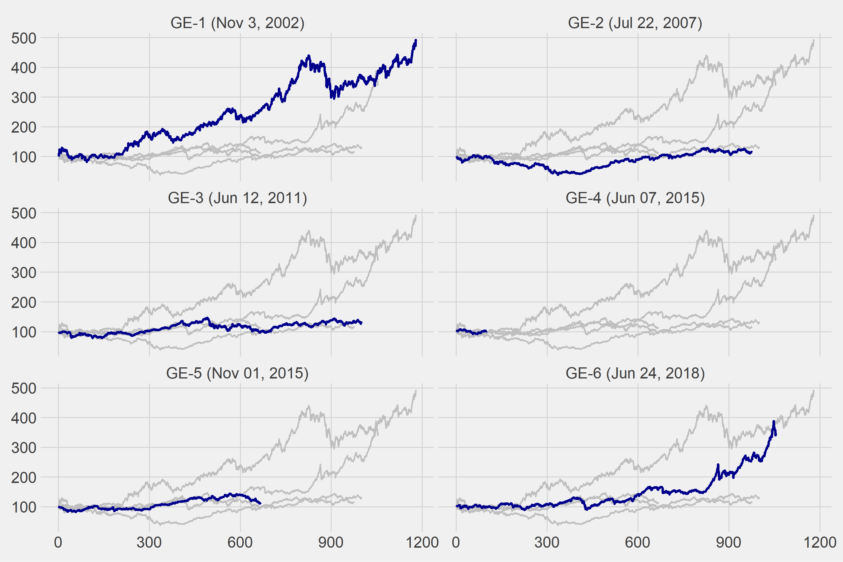
Let’s calculate the returns on a group basis.

perform100 <- master %>% 
  group_by(election) %>% 
  filter(date == min(date) | date == max(date)) %>% 
  mutate(
    return = log(1 + (lead(indices) - indices) / indices) * 100
  ) %>% 
  ungroup() %>% 
  select(election,return) %>% 
  na.omit()

election	return
GE-1 (Nov 3, 2002)	158.5
GE-2 (Jul 22, 2007)	13.6
GE-3 (Jun 12, 2011)	25.5
GE-4 (Jun 07, 2015)	2.0
GE-5 (Nov 01, 2015)	13.6
GE-6 (Jun 24, 2018)	124.9

The best performance was demonstrated between the elections in 2002 and 2007 as seen in the table above. The period following the 2018 general elections has the second best performance. Yay!

It’s too soon to celebrate! See below for the CPI values during the time of the ruling party!

cpi <- readxl::read_excel("data2.xlsx") %>% 
  mutate(
    date = lubridate::ymd(paste0(date,"-",1))
  )

ggplot(cpi, aes(x = date, y = cpi)) +
  geom_line() +
  geom_vline(xintercept = as.Date(election_dates), linetype = "dotdash", color = "red", size = 1) +
  ggthemes::theme_fivethirtyeight() +
  theme(axis.text = element_text(size = 20)) +
  scale_y_continuous(labels = scales::comma)

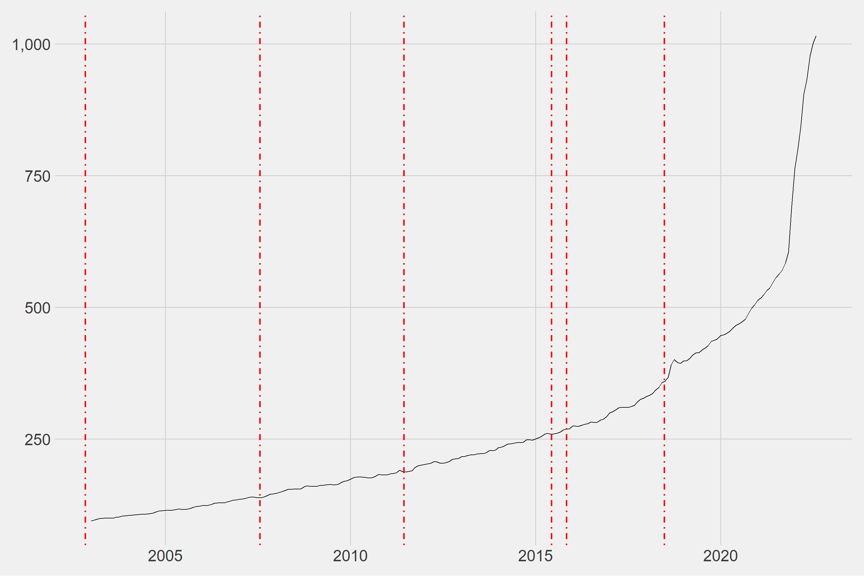
Because CPI values are published on a monthly basis, we must convert the stock market index to a monthly basis. The following formulas can be used to perform calculations.

\(P_t^{real} = P_t / CPI_t\)

\(r_t^{real} = ln(1 + R_t^{real})\)

\(R_t^{real} = (P_t^{real} - P_{t-1}^{real}) / P_{t-1}^{real}\)

bist100_monthly <- readxl::read_excel("data1.xlsx") %>% 
  mutate(date = lubridate::dmy(date),
         year = lubridate::year(date),
         month = lubridate::month(date)) %>% 
  group_by(year,month) %>% 
  summarise(close = mean(close)) %>% 
  ungroup() %>% 
  mutate(date = as.Date(paste0(year,"-",month,"-",1))) %>% 
  select(date,close) %>% 
  mutate(
    election = case_when(
      date >= as.Date("2002-11-01") & date < as.Date("2007-07-01") ~ "GE-1 (Nov 3, 2002)",
      date >= as.Date("2007-07-01") & date < as.Date("2011-06-01") ~ "GE-2 (Jul 22, 2007)",
      date >= as.Date("2011-06-01") & date < as.Date("2015-06-01") ~ "GE-3 (Jun 12, 2011)",
      date >= as.Date("2015-06-01") & date < as.Date("2015-11-01") ~ "GE-4 (Jun 07, 2015)",
      date >= as.Date("2015-11-01") & date < as.Date("2018-06-01") ~ "GE-5 (Nov 01, 2015)",
      date >= as.Date("2018-06-01") ~ "GE-6 (Jun 24, 2018)"
    )
  ) %>% 
  left_join(cpi, by = "date") %>% 
  na.omit() %>% 
  mutate(
    new_close = close / cpi, .before = close
  ) %>% 
  select(-close,-cpi)

initialValues2 <- bist100_monthly %>% 
  group_by(election) %>% 
  slice_min(date) %>% 
  rename("initial"=2) %>% 
  ungroup()

master2 <- bist100_monthly %>% 
  left_join(initialValues2, by = c("date","election")) %>% 
  mutate(initial = zoo::na.locf(initial),
         "indices" = new_close / initial * 100) %>% 
  group_by(election) %>% 
  mutate(t = row_number()) %>% 
  ungroup()

ggplot(master2, aes(x = t, y = indices)) +
  geom_line(data = master2 %>% rename(election2 = election),
            aes(group = election2), color = "gray", size = 1) +
  geom_line(color = "dark blue", size = 1.5) +
  ggthemes::theme_fivethirtyeight() +
  theme(strip.text = element_text(size = 20),
        axis.text = element_text(size = 20)) +
  facet_wrap(~election, ncol = 2)

perform100_2 <- master2 %>% 
  group_by(election) %>% 
  filter(date == min(date) | date == max(date)) %>% 
  mutate(
    return = log(1 + (lead(indices)-indices) / indices) * 100
  ) %>% 
  ungroup() %>% 
  select(election,return) %>% 
  na.omit()

election	return
GE-1 (Nov 3, 2002)	108.0
GE-2 (Jul 22, 2007)	-7.9
GE-3 (Jun 12, 2011)	-2.1
GE-4 (Jun 07, 2015)	-6.5
GE-5 (Nov 01, 2015)	-1.5
GE-6 (Jun 24, 2018)	7.0

When we consider inflation, we can see how the gap between the best return and the current period widens!