Turkey’s most developed districts were determined by the Ministry of Industry and Technology.
According to the data of the Ministry, the top 10 most developed districts out of 973 are:
| rank | province | district | score |
|---|---|---|---|
| 1 | İstanbul | Şişli | 6.959 |
| 2 | Ankara | Çankaya | 6.901 |
| 3 | İstanbul | Beşiktaş | 5.940 |
| 4 | İstanbul | Kadıköy | 4.910 |
| 5 | Ankara | Yenimahalle | 4.481 |
| 6 | İstanbul | Bakırköy | 4.465 |
| 7 | İstanbul | Fatih | 4.226 |
| 8 | Bursa | Nilüfer | 4.072 |
| 9 | İstanbul | Ataşehir | 3.545 |
| 10 | İstanbul | Başakşehir | 3.468 |
Istanbul’s Şişli named most-developed district in Turkey.
In this study, we will map the districts of Istanbul. All data can be accessed by downloading the post31.xlsx file from here.
Following is a ranking of the districts’ socioeconomic development:
df <- readxl::read_excel("data.xlsx")

df %>%
  filter(province == "İstanbul") %>%
  ggplot(aes(x = reorder(district,score), y = score, fill = score)) +
  geom_col() +
  theme_minimal() +
  theme(axis.title = element_blank(),
        axis.text = element_text(size = 15),
        legend.position = "none") +
  scale_fill_gradient(low = "red", high = "orange") +
  coord_flip()

We first download Turkey’s file from here in order to create the map. Click on the Shapefile name to download it. The zip you downloaded can be extracted and placed in your project file. There are 3 levels: level-0, level-1, and the level we are interested in, level-2.
Another option is to run the code below instead of following the steps above. The {raster} package will be used.
# raster::getData()

districts_shp <- getData(
  name = "GADM",
  country = "TUR",
  level = 2
)

class(districts_shp)
[1] "SpatialPolygonsDataFrame"
attr(,"package")
[1] "sp"
Let’s create a data frame from the file you’ll see in your environment.
# ggplot2::fortify()

districts_shp_df <- fortify(districts_shp, region = "NAME_2")

class(districts_shp_df)
[1] "data.frame"Merge the istanbul and districts_shp_df dataframes.
istanbul <- df %>%
  filter(province == "İstanbul") %>%
  rename("id"="district") %>%
  mutate(
    id = ifelse(id == "Arnavutköy", "Arnavutkoy", id),
    id = ifelse(id == "Ataşehir", "Atasehir", id),
    id = ifelse(id == "Başakşehir", "Basaksehir", id),
    id = ifelse(id == "Beylikdüzü", "Beylikduzu", id),
    id = ifelse(id == "Eyüpsultan", "Eyüp", id),
    id = ifelse(id == "Çekmeköy", "Çekmekoy", id)
  )

master <- districts_shp_df %>%
  inner_join(istanbul, by = "id")
It’s now time to map the data.
ggplot() +
  geom_polygon(data = master, aes(x = long, y = lat, group = group, fill  = score)) +
  scale_fill_gradient(low = "dark red", high = "yellow") +
  theme_void() +
  theme(
    legend.title = element_blank(),
    legend.position = "bottom",
    legend.key.width = unit(2,"cm")
  )
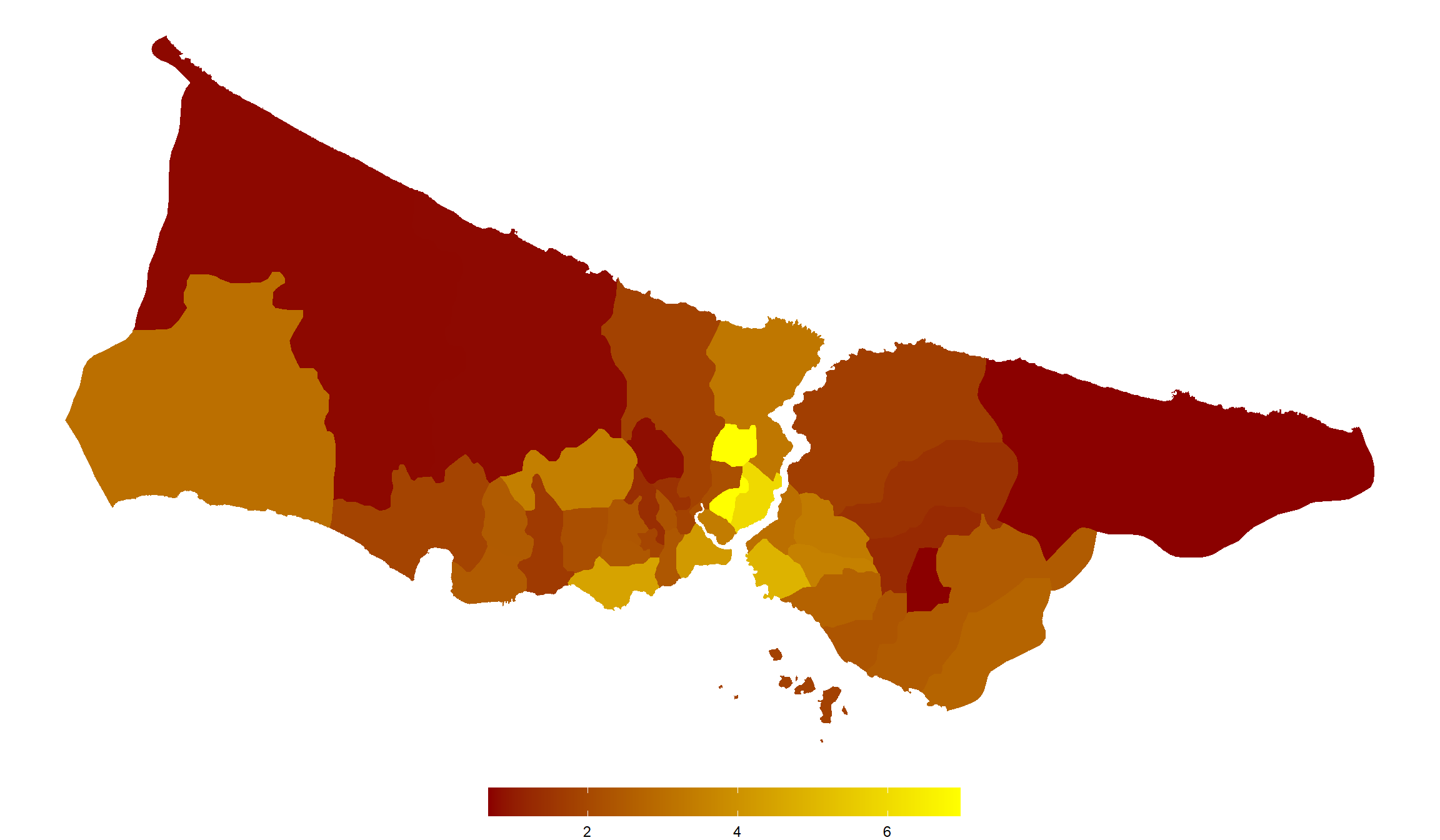
Oops! Even to someone who is familiar with Istanbul, the map appears normal, but Silivri, one of the city’s districts, is not included.
unique(master$id)
 [1] "Adalar"        "Arnavutkoy"    "Atasehir"      "Avcılar"
 [5] "Bağcılar"      "Bahçelievler"  "Bakırköy"      "Basaksehir"
 [9] "Bayrampaşa"    "Beşiktaş"      "Beykoz"        "Beylikduzu"
[13] "Beyoğlu"       "Büyükçekmece"  "Çatalca"       "Çekmekoy"
[17] "Esenler"       "Esenyurt"      "Eyüp"          "Fatih"
[21] "Gaziosmanpaşa" "Güngören"      "Kadıköy"       "Kağıthane"
[25] "Kartal"        "Küçükçekmece"  "Maltepe"       "Pendik"
[29] "Sancaktepe"    "Sarıyer"       "Sultanbeyli"   "Sultangazi"
[33] "Şile"          "Şişli"         "Tuzla"         "Ümraniye"
[37] "Üsküdar" "Zeytinburnu" istanbul$id
 [1] "Şişli"         "Beşiktaş"      "Kadıköy"       "Bakırköy"
 [5] "Fatih"         "Atasehir"      "Basaksehir"    "Beyoğlu"
 [9] "Ümraniye"      "Sarıyer"       "Üsküdar"       "Tuzla"
[13] "Maltepe"       "Beylikduzu"    "Pendik"        "Esenyurt"
[17] "Bahçelievler"  "Zeytinburnu"   "Bağcılar"      "Kartal"
[21] "Bayrampaşa"    "Kağıthane"     "Küçükçekmece"  "Güngören"
[25] "Büyükçekmece"  "Eyüp"          "Adalar"        "Beykoz"
[29] "Avcılar"       "Gaziosmanpaşa" "Çekmekoy"      "Esenler"
[33] "Silivri"       "Sancaktepe"    "Sultangazi"    "Arnavutkoy"
[37] "Çatalca"       "Şile"          "Sultanbeyli"
We leave everything behind and move on!
We went with the second option, but now we’re back to the first. With the help of the {sf} package, we’ll read a file with the .shp extension from the file we saved earlier.
I won’t change anything from what I previously told you.
istanbul2 <- istanbul %>%
  rename("NAME_2"="id")

master2 <- districts_shp2 %>%
  inner_join(istanbul2, by = "NAME_2")
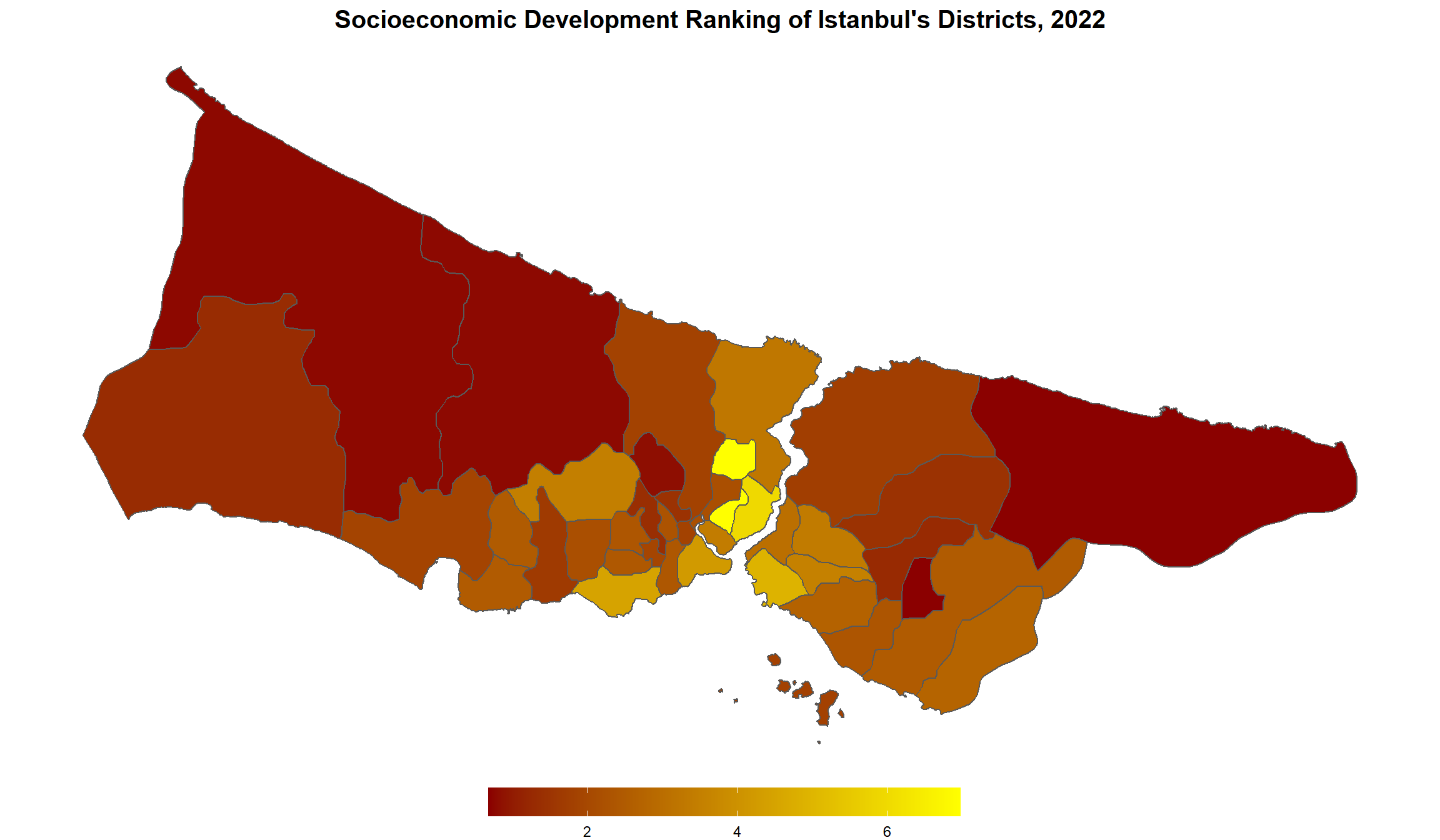
It’s now time to remap the data.
master2 %>%
  ggplot(aes(fill = score)) +
  geom_sf() +
  scale_fill_gradient(low = "dark red", high = "yellow") +
  theme_void() +
  theme(
    legend.title = element_blank(),
    legend.position = "bottom",
    legend.key.width = unit(2,"cm"),
    plot.title = element_text(size = 15, face = "bold", hjust = 0.5)
  ) +
  labs(
    title = "Socioeconomic Development Ranking of Istanbul's Districts, 2022"
  )