Although I’ll focus on data manipulation rather than the question in this post, at the end of the post we’ll have answered an important question. Let’s define data manipulation briefly before answering the question.
Data manipulation is the process of changing data to make it more readable and organized. We manipulate data in order to analyze and visualize it.
The data for this study were obtained from TURKSTAT. You can access the data by downloading post23.xls file here. The metadata can be found here.
Importing the dataset:
df <- readxl::read_excel("data.xls")I bet you can’t do analysis with this dataset! :-) In this case we convert it into an analysis-ready format.
Because annual returns adjusted for CPI will be used, the relevant columns, including the years and months, will be chosen. The column positions are in the following order: 1, 17, 33, 49, … So, 16 is the difference between two numbers that follow one another. Don’t forget the months in column 2!
| …2 | Finansal yatırım araçlarının yıllara göre dönemsel reel getiri oranları | …17 | …33 | …49 | …65 | …81 | …97 |
|---|---|---|---|---|---|---|---|
| NA | The rates of profits created by means of financial invesment | NA | NA | NA | NA | NA | NA |
| NA | NA | NA | NA | NA | NA | NA | (%) |
| NA | NA | NA | NA | NA | NA | NA | NA |
| NA | NA | NA | NA | NA | NA | NA | NA |
| NA | NA | NA | NA | NA | NA | NA | NA |
| Ay Months | Yıl Year | TÜFE CPI | TÜFE CPI | TÜFE CPI | TÜFE CPI | TÜFE CPI | TÜFE CPI |
| Ocak January | 1997 | 10 | 61.299999999999997 | 5.5999999999999996 | -3.7999999999999998 | -5.9000000000000004 | NA |
| Şubat February | 1997 | 9 | 65.200000000000003 | 4.7000000000000002 | -8 | -9.5999999999999996 | NA |
| Mart March | 1997 | 8.6999999999999993 | 31.600000000000001 | 3.2000000000000002 | -10.1 | -11.800000000000001 | NA |
| Nisan April | 1997 | 8.1999999999999993 | 25.699999999999999 | 1.8999999999999999 | -10.800000000000001 | -10.5 | NA |
The first 6 lines can be removed.
Changing column names:
The Months column contains two month names, one in English and one in Turkish. We’ll go with the English ones.
I’d like to draw your attention to the fact that there is a line break between the month names in each line. Click the icon to the left of the df2 in the environment to see it.
df2$Months[1][1] "Ocak\nJanuary"These line breaks need to be eliminated.
df2 <- df2 %>%
  mutate(
    Months = stringr::str_replace_all(Months, "[\n]" , " ")
)df2$Months[1][1] "Ocak January"Extracting the second word from each line:
df2$Months[1][1] "January"Combining month and year into a date format column and removing the Months and Years columns:
We can also remove lines that contain NA (Not Available).
We’ll convert each column to numeric format, but some values have the letter e next to them.
df2[211,6]# A tibble: 1 x 1
GoldIngot
<chr>
1 9,11(e) Let’s remove the values containing the letter “e” with their parentheses.
e: Data is corrected.
Except for the Date column, all columns can be converted to numbers.
Wait a minute! There are several values that require the conversion of commas to dots.
df2[211,6]# A tibble: 1 x 1
GoldIngot
<dbl>
1 9.11| Date | DepositInterest | StockExchange | USDollar | Euro | GoldIngot | GDDI |
|---|---|---|---|---|---|---|
| 2021-10-01 | -7.46 | 2.36 | -3.22 | -4.65 | -9.78 | -12.17 |
| 2021-11-01 | -7.72 | 9.77 | 10.35 | 6.36 | 8.06 | -13.70 |
| 2021-12-01 | -15.73 | 4.00 | 29.19 | 19.99 | 25.43 | -26.37 |
| 2022-01-01 | -22.75 | -11.67 | 23.08 | 14.45 | 19.70 | -32.69 |
| 2022-02-01 | -25.50 | -15.28 | 24.86 | 17.02 | 28.13 | -33.37 |
| 2022-03-01 | -27.73 | -12.50 | 18.14 | 9.40 | 33.59 | -35.98 |
| 2022-04-01 | -31.42 | 2.59 | 6.04 | -3.98 | 17.31 | -34.68 |
| 2022-05-01 | -32.86 | -2.17 | 8.31 | -5.60 | 8.76 | -37.08 |
| 2022-06-01 | -35.02 | 0.21 | 10.46 | -3.09 | 10.40 | -36.34 |
| 2022-07-01 | -35.26 | 0.52 | 13.06 | -2.45 | 9.11 | -34.81 |
Before performing the calculation that will take place soon, the table needs to be converted from wide to long format.
df2 <- df2 %>%
  tidyr::pivot_longer(!Date, names_to = "Types", values_to = "Returns") %>%
  arrange(Types)
Calculating the average rate of return on an investment that is compounded over several periods is possible using the geometric average return formula, also known as geometric mean return.
Geometric Average Return = \(\sqrt[n]{(1+r_1)x(1+r_2)x...x(1+r_n)}-1\)
r: Rate of return
n: Number of periods
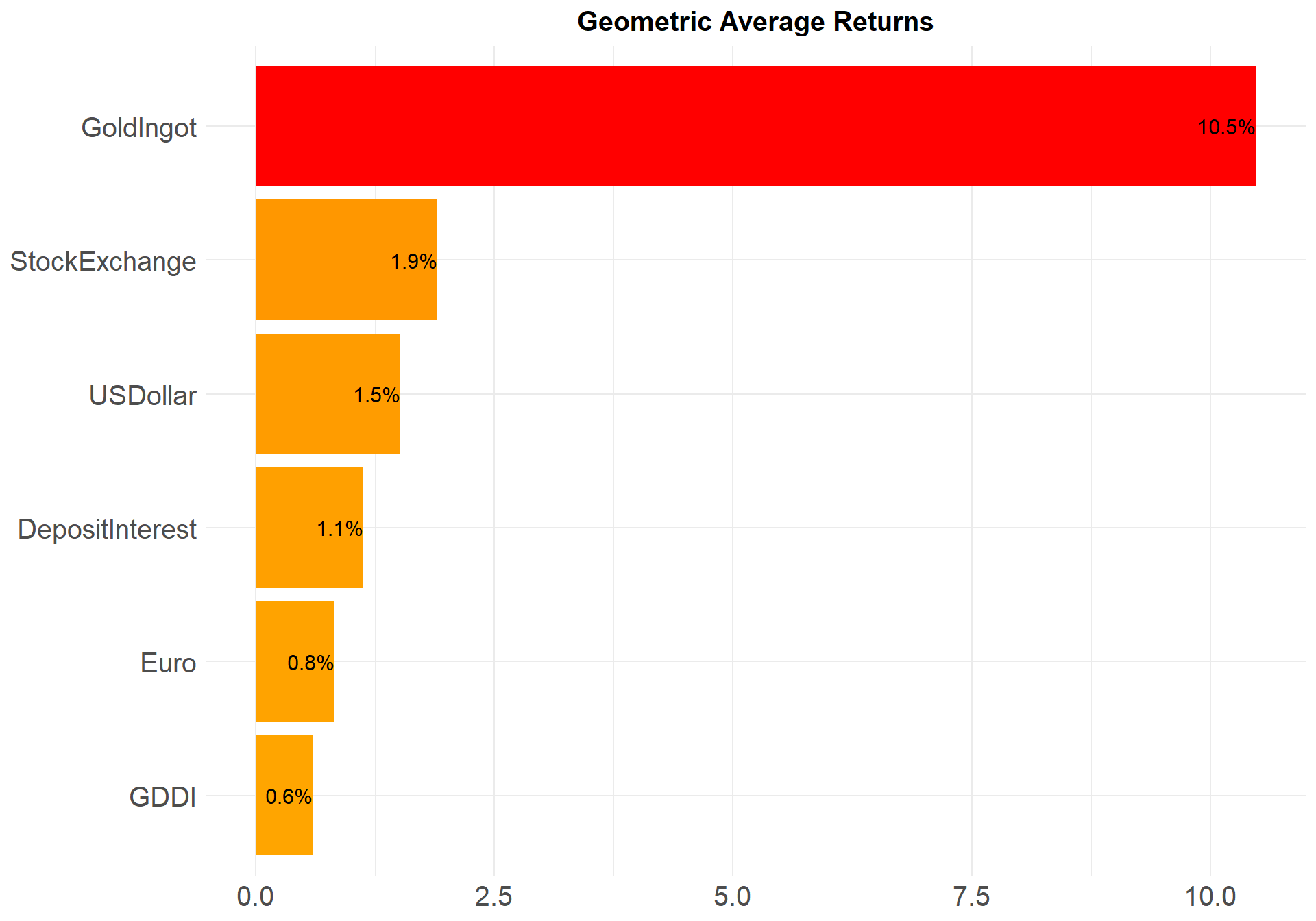
To calculate the compound average return, we first add 1.00 to each annual return. Then the above formula can be applied.
ggplot(gar, aes(x = reorder(Types,GAR), y = GAR, fill = GAR)) +
  geom_col() +
  geom_text(aes(label = paste0(round(GAR,digits = 1),"%")), hjust = 1, size = 4) +
  theme_minimal() +
  theme(legend.position = "none",
        axis.title = element_blank(),
        axis.text = element_text(size = 15),
        plot.title = element_text(face = "bold", size = 15, hjust = 0.5)) +
  scale_fill_gradient(low = "orange", high = "red") +
  coord_flip() +
  labs(
    title = "Geometric Average Returns"
  )